How it works
The technical details
How a home battery schedule becomes something a quantum computer can solve, and how I check the answers. Written as the questions a technical reader asks, so it is denser than the rest of the site on purpose.
What kind of problem is this?
What exactly goes in, and what comes out?
QAOA is the exception. It returns a distribution, not one answer. Measuring the circuit thousands of times gives thousands of candidate bit-strings with counts, each decoding to a schedule; I score them and keep the best feasible one. Identical inputs and outputs across solvers are what make the three-way comparison fair.
How do you turn a schedule into something a quantum computer can optimize?
How do you enforce the battery’s physical limits?
It is also expensive. The slack costs (T-1)·b qubits, 69 of the 117 needed for a full 24-slot day, and it dilutes the QAOA ground-state mass by 2^(T-1)b, because exactly one slack pattern pairs with the optimal decision bits. The SoC-bound penalty is pluggable (Encoding); the alternative that replaced it as the interesting default is two questions down.
Can the state-of-charge slack be avoided without breaking soundness?
Yes, and cheaply. Checkpoint pins the state of charge only every k slots and lets it float in between. Between two slots pinned to the same level and k apart, the trajectory rises at most j steps and must fall within the remaining k-j, so its excursion is bounded by max_j min(j, k-j) = floor(k/2). Whenever floor(k/2) steps of headroom exist on both sides, every zero-penalty assignment is feasible. That property is soundness: the encoding's optimum can be suboptimal, but it can never be an infeasible schedule dressed up as a bill. The spacing k is passed in and validated, never derived from the instance, because the sound ceiling depends on the initial state of charge.
Priced through the real 365-day Golden instance against the $455.72/yr the battery is worth:
| encoding | qubits | lost $/yr | infeasible days |
|---|---|---|---|
| exact | 117 | 0.00 | 0 |
| cp5band | 52 | 0.00 | 0 |
| cp3band | 62 | 0.00 | 0 |
| cp5 | 48 | 113.93 | 0 |
| cp3 | 48 | 341.79 | 0 |
| none | 48 | - | 329 (bill invalid) |
Halving the register is free; the last four qubits cost $113.93/yr. Every row in the table is lossless, which is the right basis for an encoding comparison: losses scale every row together and reorder nothing. The same $113.93 appears in docs/results/capacity-rate-sensitivity.md as the value of the 2 to 2.5 kW rate upgrade, and the coincidence is an identity rather than a transcription. Below the knee, annual value is exactly linear in delivered peak energy at $56.9646/yr per kWh/day, and both changes move 2 kWh/day: cp5 delivers 6 of the instance's 8 useful kWh/day, and the rate upgrade takes delivered energy from 8 to 10.
Two things the earlier synthetic study could not have shown.
First, the real battery (10 kWh at 2 kWh/slot) has a looser sound ceiling than the synthetic family (k up to 5 rather than 3), worth $228/yr. Capacity makes Checkpoint less conservative for free, the opposite of how the exact encoding scales.
Second, a prediction of mine that was wrong. I expected the 104 flat-tariff weekend days, worth exactly $0, to dilute annual regret below the per-day figure. They cannot: a $0 day contributes to neither numerator nor denominator. Measured regret went the other way, with cp3 losing 75% annually against 32.5% on the synthetic day. The tariff concentrates its value into a minority of high-spread days, those days need deep cycles held across many slots, and that is exactly the shape checkpointing forbids. Scaling a synthetic day would have understated the cost by more than 2x.
At T=3 the like-for-like gain is 0.00013 to 0.0453 ideal optimal mass (349x) on 6 qubits instead of 10, at 54 transpiled two-qubit gates instead of 133. Of the unsound alternatives, CenterAnchor is mis-weighted rather than useless (100% loss at the default weight, 28.79% at scale 0.001 with no infeasible days), while WindowDrift does not recover at any scale.
Is the checkpoint encoding new?
I do not know. Here is what I can say.
Adding a big cost for breaking a rule is the standard way to handle rules in this kind of problem. Paying for the battery's range with extra bookkeeping bits is the textbook version of that. None of it is mine.
What I did was refuse to pay for those bits. Pin the level every few hours instead, and prove it cannot escape in between. I worked that out on my own. I know there is research on how to handle rules like this, and I have not read it. The argument is simple enough that someone has probably written it down already.
So I am not claiming it is new. What I am claiming is what it does here, measured: 52 qubits instead of 117, the full $455.72, and it beat the exact version on hardware three times out of three.
How do you choose the penalty strength?
The penalties have to outweigh any money the solver could save by breaking a rule, or it would “cheat” by draining a battery it never filled. So I scale the penalty weights to the size of the cost itself, computed from the problem's price range by a small helper.
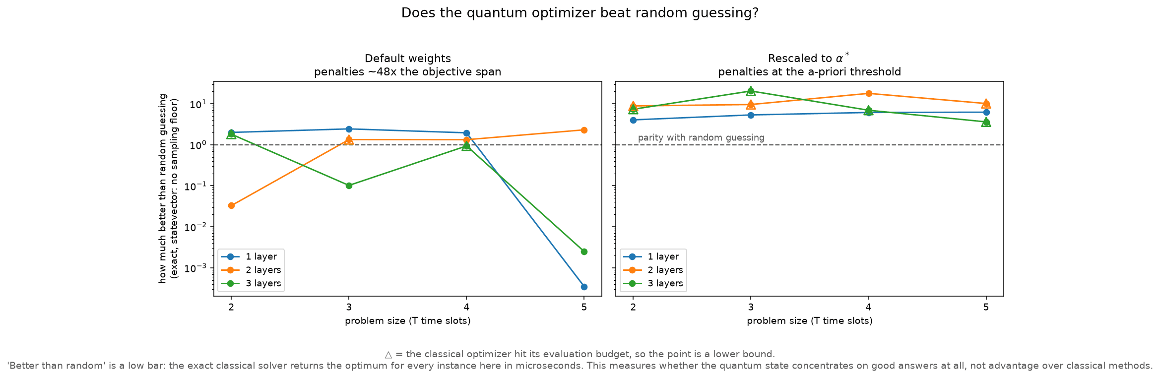
The margin in default_weights was badly wrong, and it was the dominant limit on QAOA concentration, not the encoding and not the optimizer. At T=3 it sizes penalties at 14.81 against an objective span of 0.3095 across the feasible set, a 48x overshoot. Since QAOA minimizes <H>, cost is then nearly invisible to it: reps=2 reached <H> = 1.14, which is 96.6% of the way from the uniform-superposition value to the QUBO minimum, while placing 93.6% of its mass on the feasible subspace and 0.019% on the optimum. Rescaling alone, with the encoding and the optimizer untouched, moved reps=2 ideal mass several hundredfold, from 0.00019 to between 0.073 and 0.088 depending on the alpha within the derived window, both endpoints lower bounds from capped runs.
The correct weight is derivable a priori, with no reference to any measured mass: alpha* = (objective span) / (default penalty) = 0.0209, verified at 100% optimal across 200 instance seeds at and above it and collapsing below (61% at 0.010, 6% at 0.005, 1.5% at 0.003). It supersedes the previous 10x margin.
Nothing in that ratio is specific to batteries. Any constrained problem handed to a variational algorithm as penalties plus an objective has the same failure mode: set the penalties far enough above the objective's span and the algorithm is no longer optimizing the objective, it is satisfying the constraints and calling that done. Both quantities are known before anything runs, so the check costs nothing. If you are doing this, divide the span of your objective across the feasible set by the penalty weight you were about to use, and look at the number.
Relating the penalty weight to the objective's range is an established idea with published treatments. I arrived at this ratio by measurement rather than from that work.
Does the penalty weight also control how repeatable the tuning is?
Yes, in one direction only, and the pre-registered prediction about the other direction was wrong. 1,200 tunings (10 alphas x 40 seeds x 3 instances), simulator and exact computation only, no QPU. Two tunings count as the same basin when the total variation distance between their ideal output distributions falls under tau = 0.043286, the expected shot-noise floor at 4,096 shots, recomputed at run time from 400 resamples rather than assumed. Clustering is complete-linkage, with single-linkage and tau/2 and 2*tau as pre-committed sensitivities.
The registered prediction is falsified. It was a U-shape with a strict minimum at alpha*, and the stated falsification criterion was that the basin count at alpha* is not a strict minimum over the ladder. It is not. The count is 1 at alpha* and 1 at every alpha below it, then rises monotonically above: 2 at 0.030, 3 at 0.060 and 0.100, 9 at 0.300, and 19 at default_weights. There is no lower branch. Both robustness instances reproduce the pattern and are reported rather than used to decide.
Reproducible is not correct. Basin count alone is the wrong lens, because a single basin can be the wrong basin. Below alpha = 0.010 the QUBO's minimizer is infeasible, so the search converges just as reliably onto a state that is not a schedule at all. At alpha = 0.003 the tuned circuit puts 0.0567 mass on that minimizer, higher than alpha*'s 0.0448 and worthless. Anyone reading basin count without the exactness column would conclude the low-alpha end looks fine. This was pre-registered as the main way the result could be misread.
alpha* is a boundary, not a midpoint. That is what crossing basin count with the exactness of the encoding gives, and it is the result that replaces the prediction. The usable window on this instance is 0.010 ≤ alpha ≤ 0.021, and alpha* = 0.0209 sits at its upper edge. Going 1.4x above it already doubles the basin count. The rule buys the largest penalty margin still inside the single-basin regime and nothing more, which is a warning the project did not previously have. It also sharpens the cost of the 48x overshoot: that was known to cost solution quality, and it costs reproducibility too.
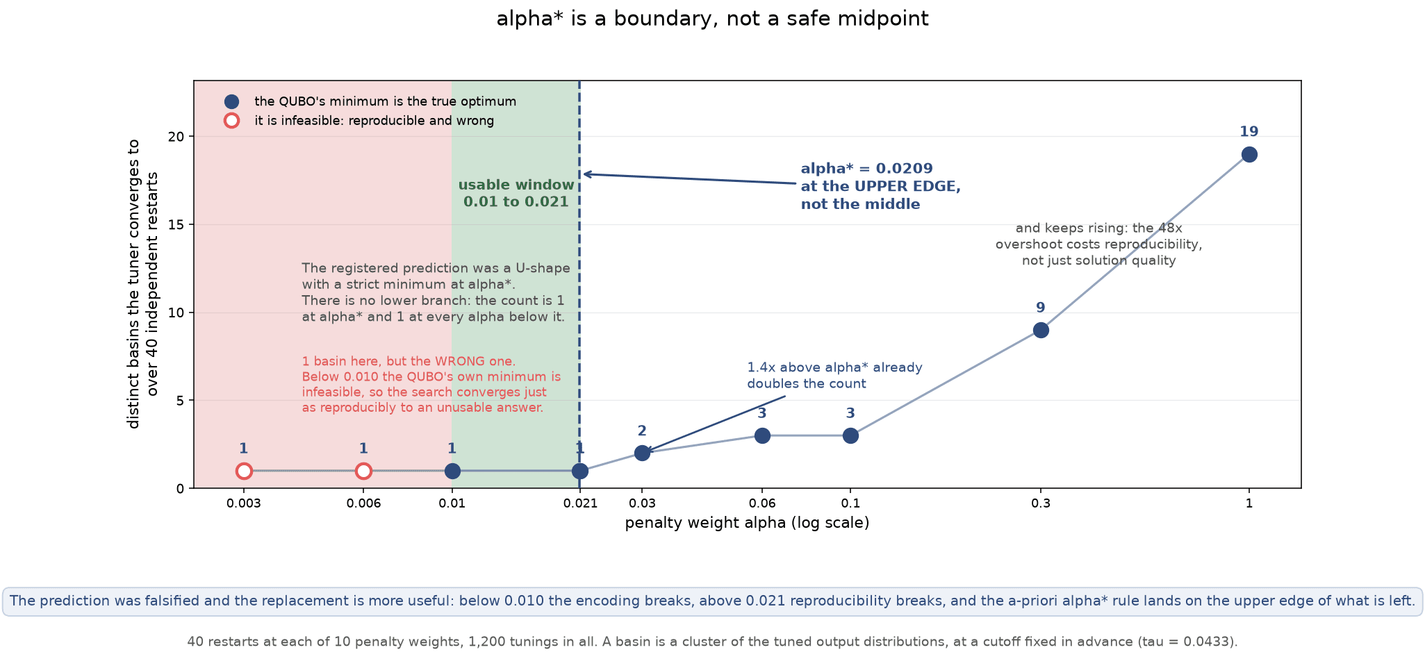
Sensitivities, all pre-committed. The count at high alpha is cutoff-dependent (22 / 19 / 13 at tau/2, tau, 2*tau), so it should be read as “many, order 10 to 20” rather than as a precise integer. The conclusion is not cutoff-dependent: every alpha at or below alpha* gives exactly one basin at every cutoff and on every instance. Complete and single linkage agree everywhere except at the default weight, where single linkage chains basins together. The window's single-basin result is stable from N=5.
One limitation is load-bearing. This is one instance family (T=3, checkpoint(3), reps=1), and nothing here transfers to reps=2, where the optimizer study's open question lives. Basin count is a property of the pinned search (n_starts=5) rather than of the true stationary-point structure. Whether any of these basins clears the 0.078125 bar is not addressed here: the best mass seen anywhere in this study is 0.0643, at an alpha where the encoding is broken. The next question takes that up at reps=2.
Does the single-basin picture survive a second layer?
No, and the same study found the first point above the concentration bar on the primary instance. Same design as the reps=1 study, registered before the sweep ran: 400 tunings (10 alphas x 40 seeds) on the optimizer study's designated instance (T=3, seed 1, checkpoint(3), reps=2), simulator and exact computation only, no QPU, tau = 0.039317 recomputed at run time. Two predictions were registered. P1, that the single-basin regime does not survive the second layer, held and not narrowly: 15 basins at alpha*, and the smallest count anywhere on the ladder is 11. P2, that no tuning at alpha* reaches the 0.078125 bar, is falsified: one of forty reaches 0.07952, at an alpha where the encoding is sound.
The operational finding is that the selection rule does not reach that tuning. The clearing tuning ranks 12th of 40 by <H>, so lowest-<H> selection (the rule QAOASolver applies, stable in N from 20 up) picks a different basin at 0.07546, 3.4% short of the bar, and a larger seed budget would not change the pick, because the clearing basin is not the lowest-<H> basin. The correlation between <H> and mass at alpha* is -0.918, so the proxy is not broken. It tracks mass through the bulk of the tunings and decouples only near the top, where the pick is made. On this instance the obstacle is selection, not existence and not budget. Whether any rule fixes that is the next question.
Two pre-committed boundaries hold. This does not reopen the optimizer budget study, which scores an arm by its mean: the mean at alpha* is 0.06379, and one clearing tuning in forty is not an arm clearing a bar. And the usable window does not transfer between instances: on this one the encoding only becomes sound at 0.0209, so alpha* sits just above the window's lower edge rather than at its upper edge. The reps=1 trap fired again on cue: at alpha = 0.006, 32 of 40 tunings clear the bar, and every one of them is mass on an assignment the battery cannot run.
Is there a selection rule that reaches the clearing tuning?
Yes, and it was sitting in the encoding's own design: keep the tuning that puts the most probability on feasible schedules, the states that decode to plans the battery can run. The penalty weight exists to push probability onto exactly those states, so this selects on whether the penalty did its job; <H> mixes that signal with the objective, and at reps=2 the mixture is dominated by the penalty term. Three pre-registered studies, simulator and exact computation only, no QPU, and all seven registered predictions across them held.
First, two fresh instances with the discovery cell excluded by construction: in all nine cells that are both sound and reproducible, feasible mass picked the single best tuning available, and on the hard instance's two rungs it cleared the bar where <H> cleared neither. Then a replication on three more fresh seeds, 1,200 tunings: the argmax pick in 12 of 12 band cells, and one of the three turned out hard, with <H>'s pick missing the bar in all three of its cells and feasible mass clearing in all three, once by only 0.00062. Then a scaling test at 8, 10, 12 and 14 qubits: the argmax pick at every size, while selecting on measured optimal mass stops working, because at 14 qubits and 4,096 shots the optimum appears in the sample for only 7 of 20 tunings.
Which rule to use depends on what is scarce. Shots cheap and the instance enumerable: select on measured optimal mass, which clears in 9 of 9 cells including the irreproducible regime where every shape rule collapses to 0.0145 or less against best masses of 0.07 to 0.14 - though on the hard instance at 4,096 shots it picks the clearing tuning 26% of the time and needs 64x the shots to reach 98%. Shots dear, or the instance too large to enumerate: select on feasible mass, which needs only a feasibility check per sample.
The size of the result. Two of the six seeds swept at reps=2 are hard, and the comparison discriminates only on those. The median margin over <H> across band cells is 5.0%, which matters only when the best mass sits at the bar. The largest size tested is still enumerable, so the scaling result probes the regime by shot budget rather than intractability. And feasible mass and lowest participation pick the same tuning in 14 of 15 held-out cells, so their agreement is one result, not two. The quantity has a published name, in-constraint probability, and the literature already uses it as a constraint inside the optimizer; the head-to-head as a post-hoc selector among restarts is the only part a day's scan of prior work did not find.
How is it solved on the quantum side?
How can my ordinary laptop imitate a quantum computer?
Because quantum mechanics, for all its strangeness, is exactly predictable arithmetic. Physics says the complete state of n qubits is a list of 2n numbers, one for each possible outcome: two qubits is a list of four numbers, and my 22-qubit test problem is a list of about 4 million. The simulator stores that list in memory. Each quantum gate is a matrix, and running the circuit means multiplying the list by one matrix after another, ordinary arithmetic. So my laptop imitates a quantum computer the way a weather model imitates a storm: nothing quantum happens inside the machine.
Interference is not faked either; it falls out of the arithmetic. The numbers in the list can be negative, so when two paths lead to the same outcome they can reinforce (+0.5 and +0.5) or cancel (+0.5 and -0.5). That canceling is interference, and QAOA's whole job of making cheap schedules likely is, on the simulator, additions where some terms carry minus signs. Measurement is just as plain: square each number to get a probability, then roll dice by those probabilities. The 4,096 draws in my results were 4,096 dice rolls.
The catch is the size of the list. Every qubit doubles it. My 6-qubit test problems need only 64 numbers, but each round of tuning updates the whole list again and again, which is why the 22-qubit simulation took about 20 to 40 minutes. At about 30 qubits, roughly a billion numbers, the list outgrows my laptop's memory. At 50 it outgrows every classical computer on Earth. At the 156 qubits of ibm_fez, the list would need roughly as many numbers as there are atoms in all of Earth's oceans. A real quantum chip never stores this list at all: its qubits are the physical state the list describes, and nature carries the bookkeeping for free. That doubling is the wall, and it is also the entire reason quantum computers might someday matter.
One more consequence: because the simulation is exact arithmetic, its qubits are perfect and noise free, the ideal machine. Real qubits are not, which is exactly why the simulator and hardware results differed, and why running on ibm_fez was the actual test.
How do you know the answer is correct?
Why compare the classical solvers by cost, not by identical schedules?
Have the checks themselves ever been challenged?
Why is the dynamic program exact and fast?
If a classical program already solves this exactly, why use a quantum computer at all?
Wait, couldn't every house just run my program itself?
Yes, and that is the right first instinct. Different homes just mean different inputs to the same easy problem, and my program solves any one of them in a tenth of a millisecond. Ten thousand independent homes is ten thousand independent solves, no quantum computer required. Any pitch that jumps from “many households” straight to “therefore quantum” is skipping something.
What it skips is that at scale the homes stop being independent. A neighborhood transformer can only carry so much charging at once, and every battery reading the same price schedule reaches the same conclusion at the same moment: charge now, it is cheap. Two hundred individually perfect plans can add up to a physically impossible one, and enough batteries chasing the same cheap hours reshape the demand pattern the prices were built on, creating a new spike at the exact moment the cheap rate begins. Once your best plan depends on what your neighbors' batteries do, the problem couples. Coupled planning is where exact classical methods hit their own exponential wall; the same doubling that stopped my laptop shows up here on the classical side.
Even then, classical computing does not give up: clever decomposition methods keep a fast per-house solver as the inner engine and coordinate the fleet around it, and they work well. The quantum bet lives at the far end, on problems so tightly coupled that even the clever classical tricks degrade, and whether quantum methods will ever win there is an open question. My one-house problem is a scale model of that coupled problem, small enough that I know the exact answer, so I can measure how far today's quantum methods actually stand from the goal. Right now, the measured distance is large.
How well does QAOA do on this problem?
Measured, not guessed: the study is committed to the repo (docs/results) as CSVs and plots, all produced on a noise-free simulator. The sweep has been run in two weight modes, and the difference between them is larger than any other effect measured here.
| T (qubits) | exact @ default | exact @ alpha* | mass ratio @ default | mass ratio @ alpha* |
|---|---|---|---|---|
| 2 (6) | 9/9 | 9/9 | 0.22 | 5.34 |
| 3 (10) | 6/9 | 9/9 | 0.25 | 7.50 |
| 4 (14) | 2/9 | 8/9 | 4.00 | 8.00 |
| 5 (18) | 0/9 | 1/9 | 64 (bound) | 64 (bound) |
Medians over 9 cells (3 seeds x 3 reps). At default_weights the median mass ratio is below parity at T=2 and T=3 (the circuit concentrates worse than uniform sampling), and exact-optimum recovery collapses with size. At alpha* = 0.0209 every measured cell beats parity by 5x to 8x and exact recovery survives to 14 qubits at 8/9. At T=5 the observed mass falls below 1/shots in 8 of 9 cells, so that row is an upper bound in both arms and no advantage is claimed there.
The yardstick is the exact probability that a single uniformly random bit-string is optimal, computed by counting optimal states (the formula the Monte Carlo regression test guards). Beyond 14 qubits the optimal mass drops below what 4,096 shots can resolve, so only upper bounds remain in either arm.
The exact dynamic program answers every one of these instances in a fraction of a millisecond. So on today's setup the quantum method is measurably better than guessing and far slower and less accurate than the classical solver, and there are now numbers that say precisely by how much. The chart further down this page shows the headline comparison.
Two qualifications on the alpha* column. First, COBYLA was capped at maxiter=200 over 5 restarts, so qaoa_evalscould never exceed 1000, and 16 of 36 alpha* cells reported exactly that. A quantity sitting on its own ceiling is not a measurement of optimizer effort; it is the ceiling. Given 5x the budget, capped cells moved ideal_opt_mass by a median of 100% against a pre-registered 10% threshold, while converged cells moved 0.0%. Censoring is a reps effect rather than a size effect: nothing is capped at reps=1 at any T, and almost everything is at reps=3. So every alpha* figure here is a lower bound: conservative rather than wrong.
Second, the metric itself had never run above T=3. Statevector(QAOAAnsatz(...)) on an un-decomposed ansatz realizes the phase separator as a single PauliEvolutionGate, which means exponentiating a 2^m x 2^m operator; that raises MemoryError inside SciPy's sparse expm at m=14. I had added, committed, and run the column, and the sweep died hours in every time, which looked like a long job crashing rather than a broken instrument. The cost Hamiltonian is diagonal, so no exponentiation is needed at all: the cost layer is an elementwise phase and the mixer a per-qubit rotation. A NumPy implementation agrees with Qiskit to 2.9e-16, handles m=22 in 5.3 s, and now cross-checks itself before the sweep spends anything.
If the simulator is perfect, why run IBM's real machine at all?
The short answer: at my problem sizes, not for the answers. The simulator computes them instantly, exactly, for free. If the goal were just the result, real hardware would add only queue time and noise.
I need it for three other things.
First, to turn a prediction into an experiment. Everything from the simulator is theory: the exactly calculated forecast of what an ideal quantum computer would do. The hardware run is the moment this project stops saying “quantum mechanics implies these statistics” and starts saying “I sent these circuits to actual superconducting qubits near absolute zero, and here is what came back.”
Second, to measure the one thing the simulator cannot contain: noise. Real qubits drift, gates misfire slightly, and readouts flip, and how much depends on the chip, the day, and the circuit. I already have the ideal distribution, so the gap between it and what the hardware returns is a number that exists nowhere except in the experiment. Comparing one layer against two on the real machine also probes a real tension, because deeper circuits should be sharper in theory but are noisier in practice. July's run did not settle it; the ordering reflected how well each circuit had been tuned more than its depth. A registered depth run on August 25 did settle it, for one small instance: I predicted a dead heat, the deeper circuit won by 4.7 times the threshold, and the identical circuits won again the next day in a fresh calibration window.
Third, because the simulator runs out. My own scaling study walked up to that wall: past about 30 qubits my laptop cannot even hold the list, and past about 50 no classical computer on Earth can. Any future where quantum optimization matters runs on hardware by necessity. So I run it at sizes where I still know the right answer.
The simulator tells me what a perfect quantum computer would do. The last question is what a real one does, and that can only be measured, not simulated.
How was the run on real hardware set up?
Three gated stages, so nothing reaches the real machine by accident:
- Tune. Set the QAOA angles on the local simulator and save them. This is done, and the parameters are committed to the repo.
- Dry run. Print the chosen backend, the transpiled circuits, the shot count (4,096), and the estimated seconds of QPU time, without submitting anything.
- Submit. Send it for real, only behind an explicit confirmation flag, so IBM's roughly ten free minutes a month cannot be spent by accident.
An analysis notebook then compares the sampled schedules from three sources (exact solver, simulator, and hardware), including the total variation distance between the distributions, to measure how much real-device noise changes the answer.
The run is also pre-registered: a document committed before any hardware results exist records the circuits (four tuned QAOA circuits, 6 to 10 qubits, on an IBM Heron device), the metrics, the interpretation rules for each possible outcome, and a falsifiable prediction: the shallower reps=1 circuit should retain at least as much optimal-state mass as the deeper reps=2 circuit, because extra two-qubit gates add device noise. The analysis pipeline was rehearsed end to end on synthetic counts, so when the real counts came back from ibm_fez they dropped into a finished report. The results are on the project page.
Three things changed for the August runs. The backend is pinned in the plan rather than chosen by least-busy, and the submit path hard-fails instead of substituting a device, because the prediction is calibrated per-device; a calibration snapshot is recorded with the counts (median 2Q gate error 0.00274, readout 0.00830 on the replication job). Transpilation moved to optimization_level=3, which on the identical July circuits cuts two-qubit gates by 8-18% (37 to 33, 77 to 71, 124 to 109, 290 to 237), a strict improvement at no cost, since device-noise TVD tracks 2Q count monotonically on exactly these circuits. And shots are set per-circuit to equalize the shot-noise floor rather than kept uniform.
An analysis defect worth recording. The first pass compared a 65,536-shot hardware distribution against a 4,096-shot simulated reference, because ideal_sim_counts defaults to the module-level SHOTS. That silently defeated the floor-equalization design in the analysis: it put exact's floor at 0.164 instead of 0.043 and inflated its TVD by 35%, which would have made the raw-gap check appear to fail. The run itself was correct; only the reference was mis-sampled. ideal_sim_for_record now exists so a plan with unequal shots samples its reference at the matching count, and the failure mode is documented at the call site rather than left as a trap.
Why did the concentration question never reach hardware?
Because its pre-registered gate was not met on the instance designated in advance. Two other experiments did go to hardware and neither is a retry of this one: the encoding-versus-degradation run covered in its own question below, and the August depth run, which flew a reps=2 circuit but measured depth on a different instance, tuned by a different rule. With the a-priori weight in place, reps=2 ideal optimal mass reaches 0.0716-0.0750 against a required 0.078125 (5x uniform at m=6), and all 12 pre-registered optimizer arm x alpha combinations fail on the primary instance. The budget ladder saturates below the bar while variance collapses (sd 0.0101 to 0.0032 to 0.0018): more starts converge on one basin rather than finding better ones. The only clearing run in the whole study came from cobyla-5, the weakest arm, so it had a worse <H> than runs that did not clear.
The result is instance-dependent, which is the pre-registration's second interpretation rule firing. On both robustness instances the same arms pass reliably: instance 2 clears 9/10 at both alphas, and instance 3 clears 10/10 with transfer at 949 evaluations against cobyla-50's 9,977. Four of six instance x alpha cells have at least one passing arm, so “QAOA concentration is the limiting factor” is not supported; seed 1, designated primary in advance, is the hardest of the three. Formally the study fails, and neither the bar nor the primary instance is reselected: picking instance 3 now, having seen it clear, is precisely the error the discipline exists to prevent. A hardware candidate at this size is plausible but needs a fresh pre-registration naming its instance beforehand. The reps=2 basin study has since located what limits this instance: the landscape contains a point above the bar, and lowest-<H> selection does not pick it. A rule that does, selection on feasible mass, has since been measured and replicated; the question above the basin studies covers it.
A separate, independent limit is transpiled gate count: T3/exact at 133 two-qubit gates would have degraded on hardware whatever the weights were. Fitting a depolarizing model to July's one usable row gives ~1.32% effective error per two-qubit gate and predicts held-out TVD at 77 and 290 gates to within 3.5% and 1%. That fit holds in sample only: three registered predictions built on the model have since missed, all by predicting more damage than the device delivers, so no forward prediction leans on it now. It also does not predict single-bitstring optimal mass for collapsed circuits, since device noise has structure and does not take the state to exactly uniform, which is why the gate is on ideal mass. T=4 and T=6 are ruled out as candidates: their reps=2 circuits (267 and about 590 gates) are past the coherence limit, and a candidate that can only run one depth cannot answer a question about depth. The 590 read 269 here until August 25, which was that circuit's one-layer count; the repository carries the correction, and the ruling-out only strengthens.
Does the QAOA objective track the thing you want?
Only partly, and the boundary is now measured. Over 500,000 random parameter vectors per alpha (the statevector evaluated directly in numpy, verified against qiskit to 4e-15), the correlation between <H> and optimal-state mass strengthens as you enter the low-energy region and then weakens sharply at the bottom: -0.396 globally, -0.576 in the best 5% band, and -0.328 in the best 0.01% band, a fall of about 40%. Mean mass rises monotonically as the band tightens (0.02894 to 0.06680) and then reverses at the refined argmin, which carries less mass (0.06570) than the mean of the best-0.01% band. The ceiling collapses too: max mass in band falls from 0.10696 to 0.07880, so the high-mass points live at moderately good <H>, not the best. alpha=0.030 behaves the same way.
The precise statement is neither “aligned” nor “misaligned”: <H> tracks mass through the bulk of the low-energy region and decouples in the final approach to the minimum. That is why stopping short scored better (cobyla-50 reached 0.0749, 14% more mass than the refined argmin), and it corrects an over-strong earlier claim of mine that no <H>-minimizing procedure could clear the bar: the best-0.01% band grazes above it at its maximum (0.07880, and 0.07947 at alpha=0.030). What holds is that the argmin does not clear it and neither does the typical near-minimum point. One asymmetry is handled deliberately: a sampled mass maximum is a valid lower bound on what is achievable, but a sampled <H> minimum bounds nothing, so the <H> side is refined by L-BFGS restarts rather than read off the sample.
Scope: all of this is ideal-simulator, T=3, checkpoint(3), m=6. The observed reps=2 > reps=1 ordering at correct weights speaks to the landscape, not to the net-of-noise question, so any future hardware pre-registration must re-derive its reps prediction from gate counts and the noise model rather than inherit it from here.
Does the slack-free encoding reduce degradation on real hardware?
Yes. The claim is pre-registered in docs/plans/hardware-run-encoding.md, and the run happened on a pinned ibm_fez for 42.0 QPU-seconds. The primary metric is a pure ordering test on normalized TVD(ideal, hardware) for the unmitigated pair; magnitude does not enter it.
| circuit | m | 2Q | shots | floor | normalized |
|---|---|---|---|---|---|
| T3/exact | 10 | 106 | 65,536 | 0.0426 | 0.3708 |
| T3/cp3 | 6 | 46 | 4,096 | 0.0497 | 0.3043 |
Shots are deliberately unequal to equalize the shot-noise floor (0.0426 and 0.0497 against a planned 0.042/0.043), rather than handing the smaller circuit an artificial edge. Same instance, same optimum, same depth, same device, same day.
Uncertainty. The estimand is TVD(ideal, hardware), and the ideal side is known exactly from the statevector, so the bootstrap (B = 10,000) resamples only the hardware counts and takes the reference as given. Raw gap 0.0516, CI [0.0375, 0.0654]; normalized gap 0.0658, CI [0.0291, 0.1013]. Both exclude zero. An earlier version reported [0.0038, 0.0977] and called the result “marginal”; that bootstrap resampled the ideal reference too, injecting noise the estimand does not contain (visible in individual CIs sitting entirely above their own point estimates), and it is retracted. Correcting it moved the lower bound eightfold.
Is the gap peakedness? If cp3's ideal distribution were relatively peakier, the normalization would under-correct. It is the opposite: cp3 occupies a larger fraction of its space (PR/D 0.572 vs 0.458) with a peak half as tall relative to uniform (2.87x vs 5.30x), so its denominator is smaller (0.3817 vs 0.4531) and the normalization penalizes it. It wins carrying that handicap, which makes the measured gap a lower bound on the encoding effect. One measure disagrees: relative entropy differs by about 2% (0.9013 vs 0.9204). That disagreement is about tail weighting rather than bulk spread, and the peakedness argument rests on the measured denominator itself rather than on any shape proxy.
Three runs, and a correction to the first two. Run 2 (five circuits, 56.0 QPU-s) gave 0.0934, CI [0.0578, 0.1290]: case A of the pre-registered table, replicated. Run 3 (twelve circuits, 48.0 QPU-s) gave 0.0448, and also measured, for the first time, the term both earlier bootstraps were blind to: ten back-to-back replicates of one circuit give sigma_total 0.02496, sigma_shot 0.01787, so sigma_device = 0.01743, 70% of the replicate spread, not a residual. Folding that in (sqrt(2)·sigma_device = 0.02465 on a one-replicate-per-arm gap) widens every published interval: run 1 becomes [+0.0055, +0.1261], run 2 [+0.0334, +0.1534], and run 3 [-0.0160, +0.1056], which no longer excludes zero. The intervals in the two prior results documents were therefore too narrow, a correction to those documents, not a reinterpretation of their data.
Pooled across the three runs: mean gap 0.0680, between-run sd 0.02437, t(2) 95% CI [+0.0075, +0.1285], all three positive (sign test p = 0.25). This interval needs no device correction: it derives from between-run scatter, which already subsumes shot noise, within-job device variance, and between-run drift, so adding sigma_device would double-count. The effect is consistently positive, small, and of the same order as the run-to-run variation, which is why three runs are the claim and no single run is. n = 3 on one device and one instance still does not establish generality.
What did that hardware run fail to show?
The noise model failed. Pre-registered magnitude bands put cp3 in [0.237, 0.349] (measured 0.3043, inside) and exact in [0.463, 0.628] (measured 0.3708, outside, below). Per the fixed interpretation rule a magnitude miss is reported as a failure of the noise model, never of the encoding result, and the headline follows the ordering. That is the model's second falsification, the mass-fitted version having already failed against July's normalized TVD.
The failure is asymmetric: implied k of 0.00789 for cp3 (inside July's [0.00587, 0.00933]) against 0.00437 for exact (below all four July circuits). Two explanations were offered and both have since been corrected:
- “Not device drift”: retracted. The argument was that drift would move both arms and
cp3sits on July's mean. Butcp3did not exist in July, so it has no baseline and “failed to move” was never observable. The replication measured drift directly with a bit-identical circuit: -0.00130, and the decomposition closes almost exactly at 43% drift, 57% weight. Both contribute; neither is claimed alone. Applying that drift tocp3puts its undriftedkat about 0.0092, still inside July's range, which is precisely why the observation looked like it ruled drift out. - “A qubit-count dependence”: retracted. July's own data shows none: m=6 mean 0.00760 against m=10 mean 0.00799, a 5% difference against a 22% circuit-to-circuit spread.
The surviving explanation is the penalty weight, via ideal-distribution flatness: at alpha = 0.021, T3/exact spreads over 2.5x as many states as at the default weight (participation ratio 469.3 vs 190.7) with a peak a third as tall (5.30x vs 16.84x uniform). A distribution already close to the device's degraded limit has less structure to lose. It is supported and it is the larger term, but the decisive test, exact at both weights on the same device with weight as the only variable, is what the replication ran, and it found drift underneath.
The secondary feasible-mass prediction was not confirmed. cp3 was predicted to retain a larger fraction of its ideal feasible mass; it retained slightly less (84.7% vs 87.9%), though in absolute terms it still delivers far more usable output (23.6% of samples vs 16.7%).
Mitigation gained nothing. Dynamical decoupling plus readout twirling made both circuits slightly worse (0.3043 to 0.3203, and 0.3708 to 0.3796). The ordering is preserved either way. The arm was declared exploratory and non-gating in advance, and the effect is small enough to sit inside run-to-run variation this design cannot resolve.
A second gate came back inconclusive, on statistical grounds. The within-job duplicate-spread gate could not be adjudicated: for two draws, sd|X1-X2| / E|X1-X2| = sqrt(2-4/pi)/(2/sqrt(pi)) = 0.756, so a single pair carries about 76% relative uncertainty and the observed 0.0389 has a plus-or-minus-1-SD band of [0.0095, 0.0683], 10% to 73% of the bootstrap gap, spanning “negligible” to “comparable”. Two separate failures, and fixing only the first would not have helped: the plan said “comparable to or larger than” without quantifying it, and I operationalized that as 50% after seeing the data; and even a number fixed in advance could not have been adjudicated at one pair per arm. Any future use of the gate needs at least three replicates, which still leaves the estimate 50% uncertain. A related claim was withdrawn too: the observed 6.3x shot-scaling against a predicted 4.0x carries roughly 107% relative uncertainty, so it is consistent with shot noise but far too imprecise to exclude a drift component underneath it.
Re-run with power, it came back INDETERMINATE. Ten cp3 replicates put sigma_device at 0.01743 against a cap of 0.361 x gap. On this run's own gap the cap is 0.01616, so the point estimate fails (ratio 0.389 against a 0.361 threshold), meaning a gap measured from one replicate per arm is not resolvable against device variance. But the 9-df interval on sigma_device, [0.0000, 0.04192], straddles the cap, so the pre-registered rule returns INDETERMINATE rather than UNRESOLVED. That is an uncomfortable split, and the rule was fixed on the interval beforehand precisely so it could not be argued afterward.
The plan also said cap = 0.361 x gap without specifying which gap. Both were computed: this run's (cap 0.01616, ratio 0.389, fails) and the pooled mean (cap 0.02453, ratio 0.256, passes). The verdict is INDETERMINATE either way, so nothing turns on it here, but the point estimate flips. That is the third consecutive plan in which an unspecified analysis choice could have decided the outcome, so stating a threshold is not enough; every quantity entering it has to be pinned too. One further retraction: an earlier draft said run-to-run variation exceeds what within-job replication explains. On 2 df the between-run sd of 0.02437 carries a 95% interval of [0.0127, 0.1532], and sigma_device = 0.01743 falls inside it, so the two are statistically indistinguishable and the data are consistent with either ordering.
How does real-world data get into the model?
Three loaders, all real and mutually coherent for Golden, Colorado:
- Solar comes from NREL's PVWatts model through its public API: given a location and a panel setup, it returns a physically modeled hourly generation profile, which I validate with sanity checks (no generation at night, plausible daytime peaks) and test offline against saved responses, so the test suite never depends on the network.
- Prices come from the OpenEI Utility Rate Database entry for Xcel Energy's Colorado Residential Energy TOU tariff (Schedule RE-TOU), flattened into an hourly $/kWh series using all-in prices, with the tariff snapshot and its caveats documented in the repo.
- Household load comes from NREL's ResStock End-Use Load Profiles: representative Colorado single-family-detached profiles bucketed by season and day type (summer and winter, weekday and weekend), about 28 kWh per day in summer and 31 in winter, packaged as local CSVs with no network calls and their derivation documented. The season boundary is pinned to the tariff's own summer months, so the load season and the price season cannot disagree.
What does the optimal plan actually save on real data?
Over a full year (PVWatts solar, RE-TOU prices, ResStock load, 5 kW panels and a 10 kWh battery in Golden, Colorado), the house with no solar and no battery pays $1,747.83; with solar and an idle battery, $777.22; with the DP-optimal battery schedule, $321.50. Solar alone accounts for $970.61 of the saving; optimal scheduling adds $455.72 of pure price arbitrage. Each schedule is also required to end its day with the battery at its starting level, so the saving cannot come from secretly spending down charge that tomorrow would have to buy back. That same constraint decouples the days, which is why the annual optimum is exactly the sum of 365 independent single-day optima and needs no coupled year-long solve.
Per day, the arbitrage is $1.93 on a summer weekday and $1.65 on a winter one.
Three caveats on those figures:
- The RE-TOU weekend schedule is flat, so arbitrage is worth exactly $0 two days a week; the whole $455.72 comes from the 261 weekdays.
- The headline assumes net metering at the retail rate. Priced at a below-retail export credit, the solar leg loses about 40% and the battery leg rises to $486.94/yr, because self-consumption earns more than exporting.
- Round-trip losses are priced: a 0.90 round trip takes the battery leg from $455.72 to $404.28/yr, and every payback figure uses the with-loss number. The dollar amounts are a tariff snapshot as of August 2, 2026, against a filed Xcel increase of about 9.9%.
How is the schedule chart generated?
What are the limits, and what is next?
With only a few QAOA layers the quantum result usually will not perfectly match the exact optimum; the scaling study above puts numbers on exactly that, and the July hardware run showed how much more the real machine's noise takes away (only the smallest circuit beat random guessing on ibm_fez). The data layer is fully real and season-coherent (PVWatts solar, RE-TOU prices, ResStock load), and the savings figure is an exact 365-day annual total rather than a single day. The encoding study is done and its claim is replicated on hardware: cp5band captures the full $455.72/yr at 52 qubits against the exact encoding's 117, cp3 degrades measurably less on real hardware at matched floors, and the penalty scaling the study exposed (alpha* = 0.0209, replacing a 48x overshoot) is the reusable result. The depth question the July run defined is now answered for one small instance: the deeper circuit wins on hardware, against my registered prediction of a dead heat, and the win replicated in a second calibration window the next day.
The project is at a stopping point as of August 2026. The open questions, in the order I would take them up:
- Scaling of the hardware advantage. The encoding result is a single ordering comparison at T=3, reps=1, on one device, now measured three times. It does not establish how the advantage scales, and the noise model's three same-direction misses show quantitative extrapolation is not yet trustworthy.
- Holiday billing. The model bills US federal holidays as ordinary weekdays, and on this tariff most of them bill off-peak like a weekend, so the annual figure overstates battery arbitrage on the 11 weekday holidays in the modeled year. The calendar rule that identifies them exists in the code and is not yet wired into the annual loop.
- The concentration question, which needs a fresh pre-registration naming its instance in advance. The uncapped re-measurement has since run and confirmed the verdict, the reps=2 basin study located the obstacle in selection, and a selection rule that clears it on every sound, reproducible cell tested is now measured and replicated. What remains is the fresh instance, and hardware.
- The within-job variance gate, which came back INDETERMINATE at ten replicates: the point estimate fails its cap and the interval straddles it. Resolving it needs either more replicates or a larger gap.
- The cost model, now closed. Asymmetric buy/sell rates and round-trip losses are both modeled. Losses cost the battery 11% ($455.72 to $404.28/yr at a 0.90 round trip). The export credit was predicted here to shrink the battery leg and does the opposite, raising it to $486.94/yr near avoided-cost through self-consumption; the solar leg loses ~40% over the same range. Payback at $11,500 is bracketed at [23.6, 28.4] years rather than bounded below, so the conclusion no longer rests on either assumption.
Measured
The scaling picture
One chart from the study: how the quantum method compares with random guessing as the problem grows.
In one line
The pipeline
Every result along the way is checked against an exact dynamic program and brute-force enumeration.
Toolkit
Tools & technologies
Classical
- Python
- NumPy / SciPy
- Matplotlib
Quantum
- IBM Qiskit
- Qiskit Aer simulator
- QAOA
Engineering
- pytest
- GitHub Actions (CI)
- Jupyter notebooks
Compute access · 2026
IBM Quantum's Open Plan is free, up to about 10 minutes of real quantum runtime every 28 days on current systems, including the 156-qubit Heron r2 processor. I develop and test on free, unlimited local simulators (Qiskit Aer) and save real-hardware time for final runs.
The short version
Back to the project
Keep reading