Project
Complete, for nowQuantum Solar Optimization
A home battery should charge when power is cheap and run the house when power is expensive. Finding the best plan for a day is a real optimization problem, the kind quantum computers are supposed to be good at one day. So I solved it properly on an ordinary computer, then took small cases of the same problem to a real quantum machine to see where that technology stands.
For most of the project I thought the quantum computer was holding my results back. It was not. The two biggest limits were mine: a setting I had chosen badly, and a measurement that never worked at the sizes I was plotting.
At a glance
Four numbers
If you read nothing else on this page.
$456
a year
What the best battery schedule is worth to a real Colorado home, solved exactly for all 365 days.
$0
for twice the battery
Once the battery holds more than it can push out during the expensive hours, the savings stop. Paying for a faster battery works, but paying for a bigger one does not.
52
qubits, not 117
A smaller way to ask the same question that gives up none of that money.
3 of 3
runs of the key comparison agree
On a real IBM machine, a three-hour version of the smaller encoding is damaged less by noise. Predicted in advance and run three times, out of the six hardware runs and 165 seconds the whole project used.
The arithmetic
Where the $456 comes from
The expensive hours are 5 to 9 PM on weekdays. The battery empties at 2 kWh an hour, so in those four hours it can put out 8 kWh, however much it holds. Each of those kilowatt-hours earns the gap between the peak price and the off-peak price. The gap is $0.20667 in winter and $0.24183 in summer, so a winter weekday earns $1.65 and a summer weekday earns $1.93. There are 175 winter weekdays and 86 summer weekdays. Multiply each gap by 8 kWh and by its day count, add the two seasons, and the year comes to $455.72. Weekends earn $0, because the weekend price is flat all day.
That is why a bigger battery earns nothing. The limit is how fast the battery can empty, not how much it holds.
My optimizer confirmed this on all 365 days. Its real job was giving me a trusted ground truth for the quantum encoding.
Start here
The whole idea, in four steps
A home with solar panels and a battery
The panels make power when the sun is out. The battery can store that power, or store cheap power from the grid, and save it for later.
Electricity prices change all day
Power is cheapest overnight and most expensive in the evening, when everyone comes home and turns everything on.
So timing is worth money
Fill the battery when power is cheap or the sun is shining. Run the house off the battery during the expensive evening hours. Same electricity, smaller bill.
My program finds the best plan
It picks the cheapest schedule for the whole day. Then I rebuilt the same problem in a form a quantum computer can attempt, to see how close it gets.
There are three choices every hour, charge, wait or discharge, and they are linked, because charging now fills the battery, which limits what you can use later. Over 24 hours that makes more than ten billion possible plans for a single day, so you cannot just try them all.
Problems with that shape are the ones people hope quantum computers will one day handle. This one is also small enough that I can solve it exactly the ordinary way, which means I always know the right answer, so the quantum machine can be graded against something already known.
The plan
What the battery does all day
One real day in Golden, Colorado, a summer weekday, from the same data as everything else here.
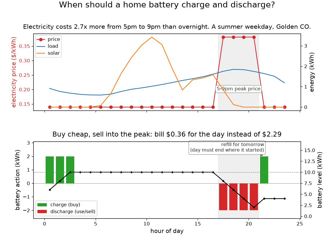
00:00 to 02:00
Charge
Power is cheapest overnight
$0.139/kWh
03:00 to 16:00
Sit full
Solar covers the house on its own
$0.139/kWh
17:00 to 20:00
Run the house off the battery
Price nearly triples
$0.381/kWh
21:00
Top back up
So the day ends where it started
$0.139/kWh
The whole strategy fits in one sentence: fill the battery when power is cheap, coast through the day on solar, and run the house off the battery through the expensive evening. A person could follow that by hand with a calendar reminder. Instead of a trick, the optimizer found the obvious thing, which is an answer anyone can check against common sense.
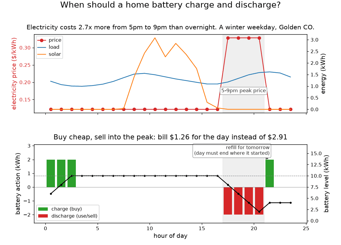
Although the prices differ and there is less sun, the winter day has the same shape, the same charging hours and the same discharging hours, and saves $1.65 instead of $1.93. The pattern is not an artifact of one day.
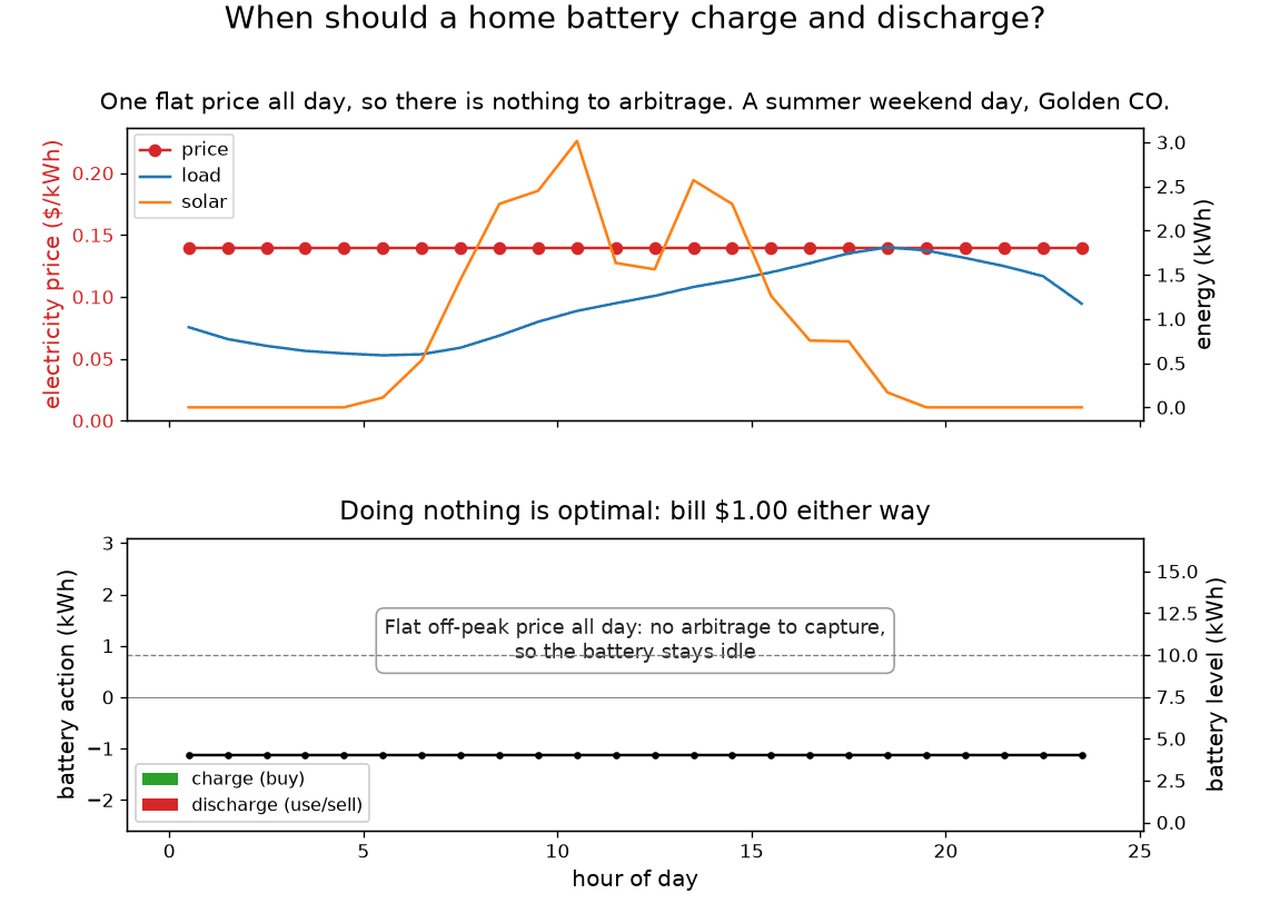
On weekends the battery does nothing at all. Because this utility charges one flat price at weekends, there is no cheap hour to buy in and no expensive hour to sell into, which makes leaving the battery alone the best possible plan. That is 104 days a year of exactly $0. A solver that reported a saving on every day would have a bug.
The clock times are arbitrary
First, the answer
What the best plan is worth
Measured sunlight, published electricity prices and real household use, for a home in Golden, Colorado.
No solar, no battery
$1,747.83
Add solar panels
$777.22
Add my program's battery plan
$321.50
Every day of the year is solved exactly and the answers are added up. That works because each plan has to end with the battery where it started, so no day can borrow charge from the next one.
All of the $455.72 comes from weekdays, because the weekend price is flat and leaves nothing to time. Timing is only worth money when prices move.
What this number assumes
What it means
What this says about buying a battery
Once I could price any battery on a real year, I could ask what changes the answer.
There is not one best schedule for that day. There are 2,448, all costing the same. Every one of them agrees on only four decisions: run the house off the battery in all four peak hours. Because the other twenty hours are a free choice, a hardware timer captures the whole value and leaves nothing for smarter software to find.
That has a consequence I did not expect. Savings rise with battery size up to 8 kWh and then stop dead: 10 kWh, 12, 16 and 20 all save the same $1.93 a day. Because the expensive hours last four and the battery can only push out 2 kWh in each of them, 8 kWh is everything it can deliver before the window shuts. The rest never moves.
Emptying faster, 2 to 2.5 kWh an hour
Same size. 2.5 is 10 kWh over four hours, so above it nothing more is earned.
+$101.07/yr
Twice the battery
Twice the storage, same speed. 10 kWh to 20 kWh.
+$0.00/yr
Speed runs out the same way, and at a place you can work out. 2.5 kWh an hour is 10 kWh divided by four expensive hours, which is the speed at which this battery just empties itself before the peak ends. Below that, part of it never gets out in time. Above it, the extra speed has nothing left to move.
So neither number is the one to shop on, because size and speed only mean anything together. Count the expensive hours on your bill, divide the battery's size by that number, and you have the speed worth paying for. The rule held on all 56 cases tested, across four different peak lengths.
Once the battery's round-trip losses are counted it saves $404.28 a year, and a $11,500 installation pays for itself in about 28 years, against a 10-year warranty. The two assumptions that used to make that a best case have both been measured, and because they pull in opposite directions the payback lands between 23.6 and 28.4 years whatever they turn out to be. Arbitrage alone does not pay for the hardware. What capacity above 8 kWh does buy is hours of power when the grid is down, which this model cannot price. Those are two different purchases sold as one number.
Try it yourself
Steer the plan
The same kind of optimizer, running live in your browser on a simplified day.
One summer weekday for a home in Golden, Colorado.
Set the battery and the evening price below. The program then searches every possible schedule of charging and discharging for those 24 hours and keeps the cheapest one.
Saved on this day
$2.56
Bill without a battery: $3.19
Bill on this plan: $0.63
The pack holds 14 kWh. Of that, 5.5 kWh goes out during the 5 to 9pm peak, because with export off the battery can only replace what the house draws while the price is high.
Sunshine and home use, hour by hour
Both in kWh. The shaded band is when electricity is expensive.
The cheapest schedule the program found
Bars are kWh into or out of the battery that hour, on the left scale. The line is how much is stored, on the right.
Raise the evening peak and the savings climb. Even at a flat $0.14 the battery still pays off, by banking free midday solar for the evening.
This is a simplified model of a day shaped like the real one. On the fully real data the battery plan is worth about $1.93 on a summer weekday, and $455.72 over a year. Which of those two settings is worth paying for is the subject of buying a battery.
The quantum part
What a real quantum computer did with it
My ordinary program solves a day of this problem in microseconds, so nothing here is a claim about beating it. The live question is whether the quantum part does anything useful yet, and how you would tell.
Each time you measure the circuit it hands back one plan, like drawing from a hat. Because a circuit that is working makes good plans come out more often than their fair share, the test is whether good plans beat random guessing.
In July I sent four circuits to ibm_fez, a 156-qubit IBM machine, for 7 seconds of machine time. Noise got worse as the circuits got bigger, as expected, until only the smallest still beat random guessing and the rest were drowned out.
That is where the technology stands today, and it pointed at what to do next. Because noise was the limit, the next step was a circuit that needs less machine.
What I did about it
Asking the same question with less than half the machine
Most of the qubits were never doing the interesting work. They were bookkeeping, bits that record the battery level every hour so the arithmetic can check it stays in range. A full day costs 117 qubits, 69 of them bookkeeping.
The version I tested checks the level every five hours instead of every hour. Although that sounds like hoping nothing goes wrong in between, it is not. The battery moves 2 kWh in an hour, so take two checkpoints five hours apart, both pinned to the same level. Whatever the level climbs in between, it has to give back before the second pin, and coming down takes as many hours as going up. Those five hours have to cover the climb and the descent together, so the climb gets at most two of them, which is 4 kWh. A 10 kWh battery has that much room above and below, so the level cannot leave its range, and no hour in between has to be checked to know that.
A plan this version accepts is always one the battery could run, so the worst it can do is pick a legal plan that costs more. The other ways I tried to drop the bookkeeping bits either lose that guarantee, handing back schedules the battery cannot follow, or keep it and lose most of the money.
Getting rid of those bookkeeping bits is an active area with published methods. I arrived at this one from the structure of my own problem rather than from that work.
Write the level down every hour
The exact method, and the one I started with.
117 qubits
Check it every five hours
Loses nothing: still worth the full $455.72 a year.
52 qubits
Drop the last four bookkeeping bits
Now it costs money: $113.93 a year of the saving.
48 qubits
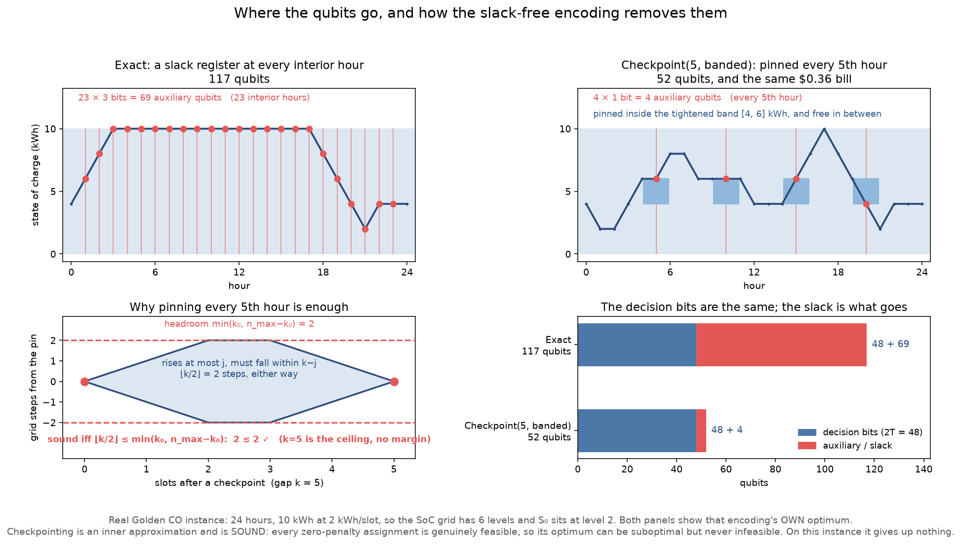
More than half the machine was free to give up. Because every version ran through the same 365 days as the exact one, the rest has a price in dollars. If a shortcut costs $113.93 a year, someone can decide whether that is worth it. These three prices are for the battery that loses nothing, which is what the encoding is compared against. Losses scale all three together and change nothing about which encoding wins.
What it gives up is real too. Because it cannot hold a charge across a checkpoint, “fill up at midday when power is cheap, sit on it, sell into the evening peak” is the one plan it rules out. Nor are more checkpoints safer, just more rigid, because every three hours instead of every five costs $341.79 a year. Every encoding tried, and what each one costs, is in slack-free-encoding.md.
Corrections
What I got wrong first
Before the result below, the things I had to take back to get to it.
The circuit has two jobs: obey the battery's limits, and among the plans that do, find the cheapest. I had set the penalty for breaking a rule 48 times larger than the whole spread between the cheapest and most expensive legal plan. Because cost was nearly invisible to the optimizer, it spent its effort finding legal plans and almost none finding cheap ones. Fixing that one number improved how often it finds the best plan by a factor of several hundred.
The chart had a second problem. Because it read its answer by sampling 4,096 times, anything rarer than one in 4,096 comes back as a flat zero. Nineteen of its thirty-six measurements were exactly that. The decline I described was my measurement hitting its own floor, not the quantum method getting worse as problems grew.
I ended up taking back four published claims, and one correction was itself an over-correction. After I found a limit distorting a measurement, I assumed the conclusion built on that measurement had fallen too, until 120 more runs showed the conclusion survived. Two of the four made my work look better and two made it look worse.
The main result
Does the smaller version actually survive better?
Fewer qubits looks good on paper. Whether it helps on hardware is a separate question.
The smaller version needs 6 qubits and 46 of the delicate two-qubit operations where the exact version needs 10 and 106. Fewer operations should mean less damage from noise, although that is a prediction, and predictions about real hardware are often wrong.
So I wrote down what I expected before running anything, then sent both circuits to ibm_fez on the same day. The measure is distance from the perfect answer, where 0 is a perfect match and 1 is completely different.
Damage on the real device, lower is better
The exact encoding
10 qubits, 106 two-qubit operations.
0.37
The checkpoint encoding
6 qubits, 46 two-qubit operations.
0.30
Same problem, same best plan, same depth, same machine. The two got different numbers of samples on purpose, so random sampling error would be equal for both rather than handing the smaller circuit a free advantage.
I checked two ways this result could have fooled me, rather than assuming them away. A gap that size could be ordinary sampling noise, so I resampled the measurements ten thousand times, and it survives. And the correction I apply when comparing circuits of different sizes could have flattered the smaller one. It runs the other way, because the smaller circuit carries a handicap and wins anyway, which makes the gap a floor rather than a ceiling.
The third way took a third run to find, and it cost me some of the result. Everything above treats the machine as steady within a job, which it is not. When I ran the same circuit ten times back to back, the answers varied on their own, by about 70% as much as the spread between whole runs.
That wobble was missing from the error bars I had already published, which made them too narrow. Corrected, the third run on its own no longer rules out zero.
So what survives
The three runs together. The smaller encoding wins all three times, and pooling them puts the effect between +0.008 and +0.129, clear of zero, which is weaker than the headline I would have written after two runs. The replication and the run-to-run spread are written up separately.
The advantage is real and consistent, although small enough that a single run cannot establish it. The scope is one problem, one size, one machine, which is enough to show the advantage exists on hardware but not to show how it scales.
The number that came out is smaller than the one I wanted.
7
jobs
33
circuits
565,248
measurements
165 s
of machine time
Split across six runs. July took 7 seconds. August 3 took 42, 56 and 48 for the comparison, the replication with a control, and the run-to-run spread. August 25 and 26 took 6 each for the depth question and its replication.
The two newest runs answered a question July could not: does a deeper circuit help once real noise is on it? I registered a dead heat and was wrong. The two-layer circuit beat the one-layer circuit by 4.7 times the pre-registered threshold, and the identical circuits repeated the win the next day in a fresh calibration window. The first run's explanation, that both depths lose the same fraction of their ideal answer, failed to replicate and is withdrawn in the write-up. The weaker claim that survives is that the deeper circuit degrades more but wins anyway, because its noise-free advantage is larger than the extra damage.
That is everything this project ever spent on real quantum hardware. I canceled a planned ten-hour run once it was clear the measurement had already bottomed out two problem sizes earlier, so it would have come back as a screen of zeros.
Verify
Check my work
Every number here traces to something you can inspect or re-run.
The hardware runs
Whenever circuits run on a real machine, IBM assigns a job ID, which my code saves with the results. All seven ran on ibm_fez:
d994b5cqp3as739tkvp0 · d9of01va5u8s73e2ljhg · d9of08bvt76s73cq0rr0 · d9og4hna5u8s73e2n26g · d9ojlotoh1qc73bc2b8g · da75ik6sidac73aetu50 · da765hk6l22c73dn5et0
Those are also collected in a provenance table with the date, shot count and device calibration for each, generated from the raw result files so it cannot drift from them. Because a job ID is only viewable from the account that ran it, the checkable part is the raw measurement counts, committed with the job IDs inside, alongside the prediction written before the run and the write-up of what came back. The plan is worth reading against the result.
The build order
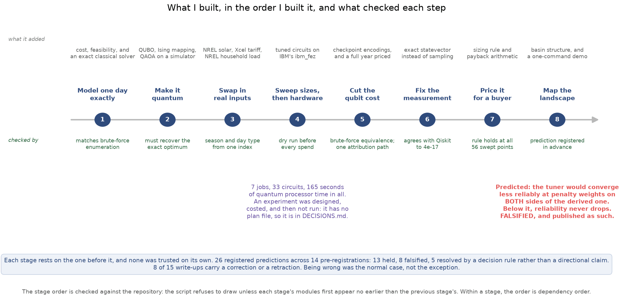
The archive
Each release of the repository is archived on Zenodo with a DOI, a permanent identifier researchers use to cite an exact version. 10.5281/zenodo.22105805 resolves to the newest version, so the numbers behind this page stay checkable even as the repository moves on.
Re-run it yourself
Four lines of setup, then one command. It prints a real day's plan, the year's three-way savings split, the sizing rule and the payback arithmetic, in about two and a half seconds, from data committed to the repository, so it needs no network and no API key. Requires Python 3.12 or newer.
terminal
git clone https://github.com/austinamissah/quantum-solar.git
cd quantum-solar
python -m venv .venv && source .venv/bin/activate
pip install -r requirements.txt && pip install -e . --no-deps
python -m quantum_solar
Then the knobs, each recomputed rather than cached: --round-trip 0.90 --export-ratio 0.25 for the realistic economics, --capacity 20 for a doubled battery earning the same $455.72, --quantum for the quantum method against the exact solvers. Every run also prints the sizing sweep, so the rate axis is on screen whichever knob you turn.
The notebook goes further, in the same environment: jupyter lab notebooks/demo.ipynb solves one instance three independent ways (brute force, dynamic programming, and the quantum method on a simulator), shows them agreeing, then plots the day. The agreement is the check that matters. Brute force is obviously correct and hopelessly slow, so it can only verify small days, which is why the fast method has to match brute force everywhere the two overlap.
If you only want to check the $455.72, the classical solvers need numpy and nothing else, because the quantum stack loads only when you ask for it.
What is new here
Three things had to be right, and one appears to be new
Getting the quantum method to work on a constrained problem took three separate things: an encoding that cannot hand back a plan the battery cannot run, a penalty weight matched to the prices, and a rule for choosing which tuning to keep. Each fails invisibly in the number you would naturally watch.
The encoding's guarantee appears to be new, and the claim is narrower than it once was. Removing bookkeeping qubits is not new, because a 2022 unit-commitment circuit removed them for the same reason and reached the qubit saving first. I learned that from a survey's reference list after my first search, and I narrowed the claim when I did. What remains mine is the guarantee. Published constructions protect the winning plan, resting on a penalty weight being set large enough, whereas mine proves that every plan scoring a perfect zero is one the battery can run, at any weight, because checking the battery every few hours bounds how far the level can drift between checks. A survey of the application area lists no encoding with that property. That is evidence from not finding something, which is weaker than finding it, and the claim is written that way where it is made. One published family, mixers that never leave the legal set, guarantees feasibility by construction. The repository records why it is an alternative and which of its costs are not measured here.
The other two are known ideas. Although deriving the penalty weight from the objective's range is established practice, what the sweep added is the price of ignoring it, measured in repeatability. The selection quantity is published under the name in-constraint probability and already used inside optimizers. The one part the search did not find is using it the way I do, which is to pick among finished tunings, head to head against the energy score.
FINDINGS.md separates the three, names the prior art, records the search's limits, and points at the test behind every number. The findings page states all three with their evidence and their limits.
Progress notes
How it got here
The turns that changed what the project claims. The full log is in the repository.
August 26, 2026
Depth went to hardware, and my prediction lost
Two registered runs, August 25 and 26, 12 QPU seconds. They asked what the July run had defined and could not answer, whether a deeper circuit helps once real noise is on it. My registered prediction, built on the noise model fitted in July, was a dead heat, which the runs falsified. The two-layer circuit beat the one-layer circuit by 4.7 times the threshold, and the identical circuits repeated the win the next day in a fresh calibration window, which is the replication the first run’s own plan required. The first run’s explanation, that both depths lose the same fraction of their ideal answer, did not survive the second run and is withdrawn in the write-up. What survives is weaker. The deeper circuit degrades more but wins anyway, because its noise-free advantage is larger. That makes three misses for the noise model, all three predicting more damage than the device delivers, so no forward prediction leans on it now. Tuning those circuits also repeated the selection-rule result on a fresh version of the problem, which is reported as an observation because it was not registered. Picking by feasible mass beat the default pick in both arms, and on the deeper arm, giving the default rule more search made its circuit worse.
August 24, 2026
A selection rule that finds the clearing tuning
Three registered studies, simulator only, following up the lost prediction below. The rule is simple: keep the tuning that puts the most probability on plans the battery can run. That rule picked the single best tuning available in every sound, repeatable setting tested, nine of nine cells on two fresh versions of the problem, twelve of twelve on three more, and four of four sizes from 8 to 14 qubits. On the two hard versions, where the best tuning barely clears the five-times-guessing bar, the energy score misses in every cell and this rule clears in every cell. Reading the answer off the sample instead stops working at 14 qubits, where the optimum appears in a 4,096-shot sample for only 7 of 20 tunings. All seven predictions across the three studies held. The limits are in the write-ups: two hard versions out of six, a median margin of 5.0 percent, and every size tested still small enough to check exactly.
August 24, 2026
Two predictions at the deeper circuit, and one lost
The deeper version of the circuit is where the open question lives, which is whether any tuning can put five times more probability on the right answer than guessing would. I wrote down two predictions and ran 400 tunings on the simulator, no quantum time. The first held, because the deeper tuning is never repeatable, with at least eleven resting places at every setting where the shallow version had one. The second lost when one of forty tunings reached the five-times bar I had predicted none would. Because the rule I use to pick a tuning goes by the circuit’s own energy score, it picks one 3.4 percent short of the bar instead, no matter how many tries it gets. So the bar is reachable on this problem, and the rule for choosing is what falls short.
August 4, 2026
A third run, and my error bars were too narrow
I had assumed a quantum computer behaves consistently within one job. It does not. Running the identical circuit ten times back to back, the answers moved on their own by about 70% as much as the spread between separate runs. That wobble was missing from the error bars I had already published, so they were too narrow. Corrected, the third run alone no longer rules out zero. What holds up is the three runs together, which is weaker than what I had after two.
August 3, 2026
The smaller circuit survives the noise better
On the machine, not on paper. I sent both versions of the same three-hour problem to ibm_fez, having written down beforehand which should win. Measured as distance from the perfect answer, the smaller encoding came back at 0.30 against 0.37, same problem, same best plan, same depth, same device. The two got different numbers of samples on purpose, so random error would be equal for both rather than handing the smaller circuit a free advantage.
August 3, 2026
The same answer on less than half the machine
Most of the qubits were bookkeeping bits, which record the battery level every hour so the arithmetic can check it stays in range. Checking every five hours instead, with a guarantee it cannot drift out of range between checks, does the same job on 52 qubits and keeps the entire $455.72 a year. Dropping the last four bookkeeping bits is where it costs something, $113.93 a year. Every version was billed through the same 365 days, so each shortcut has a measured price, not an estimated one.
August 2, 2026
A full year, not one good day
The program solves every day of the year exactly and adds up the bills. No solar or battery: $1,747.83. With solar: $777.22. With solar and my program running the battery: $321.50. The battery plan alone is worth $455.72, all of it from weekdays, because this utility charges one flat price at weekends. The whole year runs in about a tenth of a second, so there was no reason to estimate from a few typical days.
July 11, 2026
It ran on a real quantum computer
I sent the four smallest circuits to ibm_fez, one of IBM’s 156-qubit machines, for 7 seconds of machine time. Noise got worse as the circuits got bigger, as expected, and only the smallest still beat random guessing. I had also predicted shallower circuits would always survive noise better than deeper ones, which did not hold.
Go deeper
If you want the detail
Each of these is a self-contained page.
Status
Where this ends, for now
Complete as of August 2026, not finished. The code runs, the numbers can be checked, and the questions I did not get to are written down. It produced a classical result on real data, a measurement of where quantum hardware stands today, and an encoding that halves the qubit count at no cost to the answer.
Two things I would pick up first, both on the quantum side. One is whether the hardware advantage grows or fades at larger sizes, which three runs at one size cannot tell you. The other is re-running the test that missed its pre-registered bar, on a fresh version of the problem named in advance. Because shot budget and the optimization landscape have been ruled out as the obstacle, and the selection rule is now measured and replicated, the remaining suspects are the specific problem instance and the hardware.
The classical side is close to done. The model used to assume away two things, power selling back for less than power costs to buy and the energy a battery loses on every round trip. Both are modeled now, and one of them turned out to point the opposite way from what I had written. One item remains. The model bills federal holidays as ordinary weekdays, although on this tariff most of them should bill off-peak, so the annual figure overstates what the battery earns on those 11 days.